Wednesday, April 26, 2017

Quantitatve Methods

Nonparametric Statistics
- test characteristics of populations without referring to specific parameters
- designed to test ordinal data
- when data is ordinal, the mean is not an appropriate measure of central location
- does not need data to be normally distributed
- Nonparametric is distribution free statistics
- test population locations

Wilcoxon rank sum test
- compare two populations
- samples are independent
- data are ordinal or interval
- test whether population distributions are identical or not
- in locations and shapes, spreads (variances)

Sign test
- samples are matched pairs
- compare two populations of ordinal data in a matched pair

Wilcoxon signed rank sum test
- samples are matched pairs
- compare two populations of interval data in a matched pair

Kruskal Wallis Test
- compare two or more populations
- data are ordinal or interval
- data from independent samples

Friedman test
- compare two or more populations
- data are ordinal or interval
- data from randomised block experiment

Spearman rank correlation coefficient
- test whether relationship exists between two variables
- ordinal or interval data

Analysis of Variance (ANOVA)
- compare two or more population means
- by analyzing sample variance
- of interval data
- from independent samples or blocked samples
- populations are referred to as treatments

SST - sum of square for treatment
- between treatment variation

SSE - sum of square error
- within treatment variation

MST = SST / (k-1)
MSE = SSE / (n-k)

test statistics F = MST / MSE
- if F larger than Fcritical, reject H0
- if p value less than significance, reject H0

independent samples - one way ANOVA

blocked samples - two way ANOVA

Inference
- when population variance is known or given
use Z = (x̄ - u ) /(σ/√ n)
- when population variance is NOT known
use t = (x̄ - u ) /( s/√ n)

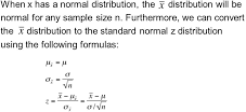
z statistics is:
and 

when z statistics is replaced by t statistics, t statistics is:
 and

use s : sample std deviation instead of population std deviation
- t stat assume data is normal

and the confidence interval estimator of u is:

- test population proportion


and

Two Populations Inference
- assume populations are normally distributed
-test the variances are equal or not
use F-test
-if variances are equal
use t-statistics
-Else if variances are unequal
use t-statistics

Chi Squared Test
- multinomial experiment
- goodness of fit test
- nominal data
- test about population's variability

Sampling and Estimation
- central limit theorem
for a large enough sample size, the distribution of sample mean is approximately normal

the probability of Z within the significance level of α
P(-Zα/2 < Z < Zα/2) = 1 -α

Example:
The student salary distribution with mean 500, variance 10
Qn: what fraction of students earn more than 520?
Ans:
P( (x̄ - u ) /(σ) > (520 - 500)/ 10 ) = P(Z > 2) = 1 - 0.9772 = 0.0228
(for population, don't need to know n)
Qn: 93.32% of students earn less than me, how much do i earn?
Ans:     find Z from 0.9332, so Z = 1.5
    then calculate    (x̄ - 500)/ 10 = 1.5  => x̄ = 515


Wednesday, April 19, 2017

SPSS independent t-test and one way ANOVA test

If you want to compare means of dependent variables on a two value variable, such as gender, you use independent t-test.

In SPSS, Click Analyze -> Compare Means -> Independent Samples T Test, a screen will pop out. In the screen, select your dependent variables as test variables , select your demographic variables, such as gender as grouping variable. You need to click the define groups button and enter 1 in group1 and 2 in group2. Then click OK and the t-test will be executed, and the independent samples test table will be shown.

On the screen, look at the Levene's Test for equality of variances.
If sig value > 0.05, look at the sig (2-tailed) upper row value. If that value is  > 0.05, the data is significant.
If sig value < 0.05, look at the sig (2-tailed) lower row value. If that value is  > 0.05, the data is significant.

If you want to compare means of dependent variables on a multiple value variable, such as age group, you use one way ANOVA.

In SPSS, Click Analyze -> Compare Means -> One Way ANOVA Test, a screen will pop out. In the screen, select your dependent variables as test variables , select your demographic variables, such as age group as factor.  Then, click on Post Hoc button, and click to enable LSD.  Then, click on Options button, and click to enable Descriptive. Then clock OK and the ANOVA test will be executed, and the multiple comparisons table, and descriptive table and ANOVA table will be shown.


Monday, March 27, 2017

CFA Level 3 - Institutional Investors

Institutional Investors
endowment annual total return = annual contribution + expense growth + management fees
(inflation is captured in expense growth)

the greater the reliance on the endowment to fund operations w/o any other sources of funds, the lower the risk tolerance of the endowment. If endowment can get donations even when it supports 75% of univ operating budget, the risk tolerance is considered high.

min return requirement of DB pension plan -> the rate that equates PV of plan assets to PV of plan liabilities, if plan is fully funded, use the discount rate to compute pernsion benefit obligation.

casualty insurance risk tolerance: uncertain loss claims by clients -> short duration, lower risk tolerance

endowment above average risk tolerance : long investment time horizon

In a defined benefit pension plan, meeting the liability is the investment objective and portfolio's benchmark.

Liability mimicking

The managers create an investment benchmark from assets that mimic the specific market-related risks associated with the pension liabilities. Then managers use derivatives to hedge the market-related exposures of the liability-mimicking assets making up the investment benchmark. This is more efficient than investing in the low risk portfolio defined by the investment benchmark because the derivatives require far less capital, thus freeing up funds. The funds can then be used for efficient return generation within asset-only space once the liabilities have been hedged. The funds invested in this asset-only space allow the pension plan to generate returns in excess of the pension liabilities, thereby decreasing the need for future cash contributions.


Investment Policy Statement (IPS) case study 


The Somchai Foundation (SF), was established to provide grants in perpetuity. SF has just received word that the foundation will receive a $45 million cash gift three months from now. The gift will greatly increase the size of the foundation’s endowment from its current $10 million. The foundation’s grant-making (spending) policy has been to pay out virtually all of its annual net investment income. Because its investment approach has been conservative, the endowment portfolio now consists almost entirely of fixed-income assets. The finance committee understands that these actions are causing the real value of foundation assets and the real value of future grants to decline because of inflation effects. Until now, the finance committee believed it had no alternative to these actions, given the large immediate cash needs of the research programs being funded and the small size of the foundation’s capital base. The foundation’s annual grants must at least equal 5 percent of its assets’ market value to maintain SF’s tax-exempt status, a requirement that is expected to continue indefinitely. The foundation anticipates no additional gifts or fundraising activity for the foreseeable future.


Given the change in circumstances that the cash gift will make, the finance committee wishes to develop new grant-making and investment policies. Annual spending must at least meet the 5 percent of market value requirement, but the committee is unsure how much higher spending can or should be. The committee wants to pay out as much as possible because of the critical nature of the research being funded; however, it understands that preserving the real value of the foundation’s assets is equally important in order to preserve its future grant-making capabilities. You have been asked to assist the committee in developing appropriate policies.

Identify and discuss the three key elements that should determine the foundation’s grant-making (spending) policy.

Formulate and justify an investment policy statement for the foundation.

Answer:
Three key elements:
  • expected inflation
  • expected nominal return
  • the 5% min payout requirement to maintain tax exempt status

IPS (Investment Policy Statement)
return objectives:
the foundation must maintain the real value of its capital, after grants. The minimum return requirement should be spending rate + expected inflation + management fee
risk objectives:
based on long time horizon and low liquidity need, the foundation's risk tolerance is above average.
liquidity needs:
low 
time horizon:
foundation has long time horizon, unlimited life span
tax considerations:
tax exempt if annual spending more than 5% of its assets' market value
legal and regulatory constraints:
the foundation is governed by IRS and UMIFA regulations.
unique circumstances:
none

Friday, March 24, 2017

CFA Level 3 - Fixed Income Portfolio Management

Managing funds against a bond market index benchmark
- Pure bond indexing
- Enhanced indexing by matching primary risk factors
- Enhanced indexing by small risk factors mismatches
- Enhanced indexing by larger risk factors mismatches
- Active management by larger risk factor mismatches
- Full blown active management

Managing funds against liabilities
- Immunization: locking in a guaranteed return over a particular horizon
1) single period immunization (classical immunization). It requires offsetting price risk and reinvestment risk. It can be done by duration matching (matching the duration of portfolio to liabilities)

for upward sloping yield curve, the immunization target rate of return < ytm because of lower reinvestment return. (price risk -> high yield lowers bond prices, price change is more than the increase in reinvestment of coupons )

type of risks:
interest rate risk, contingent claim risk (mortgage back securities when underlying mortgage prepay principal), cap risk (asset return are capped)

2) Multiple liabilities Immunization: composite return of portfolio equal composite return of liabilities

- Cash flow matching
match liability flow with assets flows of the portfolio. Immunization require less money to fund liabilities

Duration hedging
Basis risk : the difference between cash price and futures price is called basis, risk that basis will change is called basis risk
Unhedged position - has price risk, which is a risk that cash market price will move adversely
A hedged position substitute basis risk for price risk

hedged ratio = Factor exposure of bond to be hedged/factor exposure of hedging instrument
= (DT-DI)PI/DCTDPCTD * conversion factor of CTD bond

Derivative Strategies
-interest rate future
-interest rate swap: dollar duration of swap = dollar duration of fixed rate bond -  dollar duration of floating rate bond
-interest rate options
-credit risk instruments

International bond investing
 Δ in value of foreign bond = duration * Δin foreign yield given change in domestic yield
 Δ in value of foreign bond = duration * Δin yield * country beta

Duration definition
Macaulay duration: weighted average time to receive of CFs, using PV of each CF as the weight on time until it is received
Modified duration: % Δ bond price  for 1% Δ in the its ytm, assuming CFs don't change
Effective duration:  % Δ bond price  for 1% Δ in the its ytm, assuming CFs might change
spread duration:  % Δ bond price  for 1% Δ in its spread over treasury of same maturity
key rate duration: % Δ bond price  for 1% Δ in the ytm of treasury of a given maturity

Duration of Foreign bonds
adjusted duration = county duration * country beta
ΔPrice = adjusted duration * Δyield
Contribution = % weight * adjusted duration

Important points
As interest rate changes, portfolio duration will change (look at the price yield curve), portfolio must be re-balanced to adjust duration to desired level.

Portfolio can be managed to generate additional returns, the incremental difference between min return and higher possible immunized rate, is known as cushion spread. When there is cushion spread, manager can actively manage part of the portfolio. Contingent immunization is to integrate immunization strategies within active mgt strategies.

When manager expects credit spread will widen due to economic worsening, curve adjustment trades take place. The strategy is to shift the portfolio exposure to shorten the spread duration by buying shorter maturity bonds, and sell longer maturity bonds, and lower the contribution to spread duration

To immunize portfolio target yield against change in market yield, the bond portfolio must be (1) duration = investment horizon (2) Initial PV of all CFs = PV of future liability

Given a upward sloping yield curve, bond's ytm increase as maturity of the bond portfolio increase. A long duration portfolio will fall more in price than the short duration portfolio.

Hedging of foreign bonds
Example: domestic currency USD, holds Euro denominated bonds, Euro rate 2.50% US rate 0.25%

According to IRP, USD appreciates by 0.25%-2.50% = -2.2.5% (Euro depreciates)

expected depreciation of euro is 1.75%.

There is no need to hedge in this case.


Thursday, March 23, 2017

Working Capital

Operating capital: capital used in daily operations of a business
Working capital: includes inventory, cash, raw materials, and A/R
Net Operating Working capital: measure operating liquidity of a business

NWC = CA - CL
NOWC = (CA - Cash) - CL
NWCInv (for calculating FCF) = does not include cash, cash equivalent, notes payable and current portion of debt

CA are Inventory, A/R, Prepaid expense
-- Cash, marketable securities are considered non-operating assets, not included in CA
CL is A/P, Accruals, non interesting bearing liabilities
-- Notes payable is not included in CL


When finding the net increase in working capital for the purpose of calculating free cash flow, we define working capital to exclude cash and cash equivalents as well as notes payable and the current portion of long-term debt. Cash and cash equivalents are excluded because a change in cash is what we are trying to explain. Notes payable and the current portion of long-term debt are excluded because they are liabilities with explicit interest costs that make them financing items rather than operating items.


Tuesday, February 28, 2017

Microeconomics

Economic Optimization
Total revenue
TR = f(Q)
TR = P * Q
MR = 𝛿TR/𝛿Q

Revenue maximization
TR = f(Q)
dTR/dQ = 0
when MR = 0, revenue is max

Average cost minimization
MC = dTC/dQ
AC = TC/Q
set MC = AC, solve for Q

Profit maximization
π = TR - TC
π(Q) = TR(Q) - TFC - TVC(Q)  
dπ/dQ = dTR/dQ - 0 - dTVC/dQ = 0    ; if ignore TVC
dπ/dQ = 0    -> mπ = 0
dTR/dQ = 0 -> mR = 0
So: mπ = mR

π(Q) = TR(Q) - TC(Q)
dπ/dQ = dTR/dQ - dTC/dQ = 0
marginal profit
Mπ = MR - MC = 0
Mπ = 0 , MR-MC = 0
So: MR = MC

Accounting profit πA = TR - TC(explicit)
Economic profit πE = TR - TC(explicit + implicit)
πE = πA - implicit cost(opportunity cost)

In perfect competition, business are earning normal profit, and economic profit is zero.

πE = 0
Normal profit = TC(explicit + implicit)

Demand Analysis
Market basket: combination of good and services that gives the same amount of utility or satisfaction

Indifference curve:
A curve of all market baskets that provides same utility to consumer
indifference curves do not intersect, convex to the origin, slopes downward

A->B->C, the utility value of one unit of x becomes smaller compared to y, then the amount of x to substitute is larger
(the more unit you consume, the less satisfaction per unit you get)

Budget constraints
B = PxX + PyY
slope of B  = dY/dX
PyY = B - PxX
Y = B/Py - Px/Py X
slope of B = dY/dX = -Px/Py
combination of products that can be purchased for a fixed amount

Income effect: increase in consumption after price cut

Substitution effect: changes in consumption as consumer substitute cheaper products for expensive ones

Effect: The change of relative prices is the substitution effect (steep line to dotted line) and the change of purchasing power is the income effect (dotted line to parallel solid line)

Engle Curves:
The effects of changing income on consumption

Optimal Consumption
for utility max, slope IC = slope B
-MUx/MUy = -Px/Py
MUx/Px = MUy/Py

one dollar you spend on goods X, give you the same satisfaction or not, compared to one dollar you spend on good Y

Marginal rate of substitution (MRS)
MRS = dY/dX, slope of an IC
MUx = dU/dX
MUy = dU/dY
MUx*dX = -MUy*dY
slope IC = dY/dX = -MUx/MUy = MRSxy

MRSxy = MUx/MUy

On the consumption side, for utility to remain constant, the quantity goods X has to be given up for one extra unit of goods Y.

Elasticity
Point elasticity
 e = %ΔY/%ΔX = X/Y * DY/DX
Arc elasticity
E = ((Y2-Y1)/((Y2+Y1)/2)) / ((X2-X1)/((X2+X1)/2))

Price elasticity of demand = %ΔQ/%ΔP
Point elasticity
 e = (P/Q) * (DQ/DP)
Arc elasticity
E = ((P2+P1) / (Q2+Q1) ) * ((Q2-Q1) / (P2-P1))

completely inelastic demand, ep = 0, see below
completely elastic demand, ep = infinite
(happen in perfect competition market, price taker only)

Price elasticity and price changes
elastic demand  |ep| > 1.0
  luxury goods  %ΔQ>%ΔP
  P↓ => Q↑ ->  P↓ => TR↑
  P↑=> Q↓ ->  P↑ => TR↓
unitary elasticity |ep| =1.0
inelastic demand |ep| < 1.0
  necessity goods  %ΔQ<%ΔP
  P↓ => Q↑ ->  P↓ => TR↓
  P↑=> Q↓ ->  P↑ => TR↑


Production Analysis
Marginal Product
MPx = dQ/dX

Isoquant
Different input combinations used to efficiently produce a output

Marginal rate of technical substitution
MRTSxy = MPx/MPy

On the production side, for output to remain constant, the quantity input X has to be reduced for one extra unit of input Y.

imperfect substitution
perfect substitution
perfect complement
Margin revenue product
MRPx = dTR/dX = dQ/dX * dTR/dQ
          = MPx * MRQ

Margin revenue product of Labor
PL = MPL * MRQ =  MRPL
PL is wage of labor

If MRP > MC, profit will increase
Economy efficiency MRP = MC

Budget line (isocost curve)
B = PxX + PyY
slope of B  = dY/dX
PyY = B - PxX
Y = B/Py - Px/Py X
slope of B = dY/dX = -Px/Py

Expansion path
for utility max, slope Isoquant = slope B
-MPx/MPy = -Px/Py
MPx/Px = MPy/Py

Output elasticity  = %ΔQ/%ΔX
Point elasticity
 e = (X/Q) * (DQ/DX)
Arc elasticity
E = ((X2+X1) / (Q2+Q1) ) * ((Q2-Q1) / (X2-X1))

Degree of operating leverage (DOL)  = %Δπ/%ΔQ
 e = (Q/π) * (Dπ/DQ)
DOL = (P-AVC)/(P-AC)

Cost Analysis
TC = TFC + TVC
AC = AFC + AVC
MC = dTC/dQ
short run cost curves
Profit contribution πc
πc = P - AVC  per unit
πc = PQ - AVC*Q  total
      = TR - TVC
P > AVC => π+
P < AVC => πc  -

Learning curve


learning rate  (AC1 - AC2) / AC1 *100

Breakeven analysis
total  revenue = total cost
  P * Q = TFC + AVC * Q
  QBE = TFC / (P - AVC)

Cost elasticity  = %ΔTC/%ΔQ
Point elasticity
 e = (Q/TC) * (DTC/DQ)
Arc elasticity
E = ((Q2+Q1) / (TC2+TC1) ) * ((TC2-TC1) / (Q2-Q1))

Price Theory
Competitive markets
P = MR = MC

Imperfectly competitively markets
TR = PQ
MR = dTR/dQ = d(PQ)/dQ
       = PdQ/dQ + QdP/dQ
       = P(1 + Q/P * dP/dQ)
MR = P(1 + 1/ep)
max π: MR = MC
P* = MC/(1 + 1/ep)   -> P* is profit max price per unit

MOC = (P-MC)/MC => P=MC(1+MOC)  ; markup on cost
Optimal markup on cost = -1/(ep+1)

MOP = (P-MC)/P)  ; markup on price
Optimal markup on price = -1/ep

Competitive Market
- essential identical products
- large number of buyers and sellers
- free entry and exit
- opportunity for normal profits in the LR (LR: P = MC = AC)


SR: MC is the supply curve.
P=MC=MR (point A)
π= TR - TC  = rectangle CBQ1


LR: MC is the supply curve.
P=MC=AC
π=0

Monopoly
- product has no substitutes
- only one seller
- restricted entry and exit
- opportunity for economic profits in the LR (LR: P > AC)
- pricing power


For SR and LR , P > Cost, monopoly equilibrium Q is at MR = MC. MC is the supply curve.

For deadweight loss, it occur because P > Cost and Qm < Qc.

social benefits of monopoly
- economies of scale
- invention and innovation

Monopolistic Competition
- differentiated products
- many buyers and sellers
- free entry and exit
- opportunity for normal profits in the LR (SR: P > MC, LR: P = AC)

when P=AC,  there are normal profit , but zero economic profit

Qn: compare perfect competition and monopolistic competition, why perfect competition is more efficient in the LR?
- perfect competitive market P= AC at the lowest AC
- monopolistic competition P = AC , but that AC is not the lowest AC
- so perfect competition is more efficient than monopolistic competition

Oligopoly
- identical or differentiated products
- interdependent price output decisions
- few competitors
- opportunity for economic profits in the LR (P > MC, P = AR > AC)
- restricted entry and exit
- output setting models (cournot, stackelberg)
- price setting models (sweezy, bertrand)

Cournot model
- firms make simultaneous and independent output decisions
- duopoly, two firms
- find output reaction curve

Stackelberg model
- sequential output settings, big firm set output levels, smaller firm follows
- price leadership
DL = DT -Sf , DT is total demand, Sf is follower supply curve
Price leader faces demand curve DL, as a monopolist, max profit where MRL = MCL, at Q1 and P1. Followers supply output of Q3 - A1.

Bertrand model
- firms make simultaneous and independent price decisions
- find price reaction curve

Sweezy model
- kinked demand curve

This model faces a kinked demand curve, indicating that competitors will react to price reductions by cutting their own prices and causing the segment of the D curve below the kinked to be relatively inelastic. Price increases are not followed, causing the portion of the D curve above the kink to be relatively elastic.


Wednesday, February 22, 2017

Macroeconomics (Part 1)

Short Run

Closed-economy IS-LM model, which focuses only on the relationship between the interest rate and output. Assume price is fixed.

Equilibrium Output
The 45 degree line means production and income are equal. The demand curve is
ZZ =  C + I + G = c0 + c1(Y-T) + I + G = c0 -c1T + I + G +c1Y
ZZ = autonomous spending + c1Y

 autonomous spending is the intercept with vertical axis
 c1 is the propensity to consume

Equilibrium happens when demand = production.

Goods Market
Y = C + I + G  and S = Y - T - C = I + G - T
so  S + T = I + G
if G = T => S = I

Financial Market
demand for money, depends on income and interest rate
  Md = $Y L(i)              $Y+  , L(i)-
A rise in income leads to rise in demand for money
A rise in interest leads to decrease in demand for money
intersection of money supply and money demand is equilibrium interest rate.
real money supply = real money demand
  Ms/P = Y L(i)

CB control currency and reserves
  high powered money (monetary base) = currency + reserves

Let CU be currency, D demand deposit, M money supply, c is proportion of money in currency, H is monetary base, θ is reserve ratio
M = CU + D ;  CU = cM ; D = (1-c)M ;  R = θD
H = CU + R
M =  (1/(c + θ(1-c))) H

Q: Can CB closely control the money supply?
Ans: No, CB control H and θ, but cannot control c, so CB cannot closely control money supply

zero lower bound: nominal interest rate cannot go below zero
liquidity trap: when nominal interest rate  is zero, monetary policy cannot lower it further, implying monetary policy is not effective

Goods Market in open economy

ZZ: demand for domestic goods
AA: domestic demand for domestic goods
DD: domestic demand for goods

As income goes up, some additional domestic demand falls on imports. So AA is flatter than DD. Exports do not depend on domestic income, AA and ZZ have some slope.

As income (output) goes up, imports increase, exports do not change. So NX decrease.

Medium Run

Medium run: 1) price can change 2) include labor market

Labor market:
Wage setting: W = PeF(u,z)          ; z: catchall variable for all other variables
Price setting P = (1 + m) W          ; m: mark-up of price over wage

equilibrium in labor market: F(u,z) = 1/(1+m)

Original Phillips Curve
π= π-  expected inflation is rather constant
         _
π = π+ (m + z) - αut

So, negative relationship between unemployment and inflation.
Original phillips curve implies there is no natural rate of unemployment

Modified phillips curve
from P = (1 + m) PeF(u,z)
let F(u,z) = 1 - αu+ z             ; α:  strength of unemployment on wage
P = (1 + m) (1 - αu+ z)

so  after maths transform:πt - πt-1 = (m + z) - αut

if  0 = (m + z) - αu and so the natural rate of unemployment is

un = (m + z) /α

Phillips curve and the natural rate of unemployment
πt - πt-1 =  -α(u- (m + z)/α)
let un = (m + z)/α ; un : natural rate of unemployment
πt - πt-1 = - α(ut - un )


Implications:
The natural rate of unemployment is the rate that keep inflation rate constant, or we call this rate NAIRU - non accelerating inflation rate of unemployment

Not sustainable to keep unemployment rate below un, because if you do that, inflation gonna rise

Short to Medium Run : The IS-LM-PC model

Modified phillips curve
πt - πt-1 =  (m + z) -  αut

πt - πt-1 = (α/L)(Y - Yn )             ; L: labor force size

Yn is potential output, so when output is above potential output, inflation rises

IS-LM in equilibrium in the short run, but output is above potential output, so inflation rises, or economy overheating

A rising inflationary pressure makes central bank raise the policy rate. The at medium run, Y and r are at natural levels and inflation rate may not change.

Zero lower bound:
Economy in recession, and output gap is negative (Y - Y< 0).
Central bank need to reduce real policy rate to restore Y to Yn and make inflation stable. But, zero lower bound constraint make it impossible to achieve a negative real policy rate.

Central bank controls nominal rate only.

deflation and negative output gap feed on each other. Lower output leads to more deflation, more deflation lead to higher real interest rate and lower output.

Long Run

Production function: Y = F (K,N)
assumed to be constant returns to scale, if K and N are doubled, output will also double.

Y/N = F(K/N, 1)         K - capital, N - worker
If only one factor of production is doubled, the output less than double (decreasing returns to scale)

In the interactions between output and capital, there is a steady state, as shown by equation below
  sf(K*/N) = 𝛿(K*/N) or s(Y*/N) = 𝛿(K*/N)
where s: saving , 𝛿: depreciation


It is interpreted as, additional machines invested = machines that are depreciated.

If savings > depreciation, Yt/N will rise as depicted in diagram below.

The golden rule level of consumption is the saving rate that yields the highest level of consumption in steady state.


We have endogenous growth mode, where a steady growth is achieved without technological progress. The model indicates that in the long run, growth rate depends on savings rate and rate of spending on education.

To include technological progress effect on rate of growth, let
 Y = F(K, N, A)  where A: tech, K: capital, N: labor
 Y = F(K, AN)   another form
 Y/AN = F(K/AN, 1)
or Y/AN = f(K/AN)  output per effective worker is a function of capital per effective worker
Let I = S = sY
I/AN = sY/AN
The gA is growth rate of technology progress
The gN is growth rate of workers

The above graph says output per effective worker (Y/AN) and capital per effective worker (K/AN) converge in the long run.

I = 𝛿K + (gA + gN)K  = (𝛿 gA +gN)K
I/AN = (𝛿 gA +gN)K/AN

At steady state :
Y/AN, K/AN  the LR growth is 0
Y/N, K/N       the LR growth is gA
Y, K               the LR growth is gA + gN

Expectations

IS relationship
Y = C(Y-T) + I(Y, r+x) + G
A(Y, T, r, x) = C(Y-T) + I(Y, r+x)            A:aggregate private spending
Y = A(Y, T, r, x) + G
adding expected values of future variables
Y = A(Y, T, r, Ye, Te, re) + G

The effects of expansionary monetary policy and expectation
Without expectation, monetary expansion would lead to a fall in policy rate from r to r" and output rises from YA to YB. WIth expectation, IS also shifts right and output rises from YA to Yc.

Budget deficit reduction
SR: A -> B, Y0->Y1  lower spending and lower output
MR: r↓ , Y1 -> Y0  due to lower interest rate, unchanged output, higher saving and higher private investment (Because output unchanged, gov spending is reduced, so private investment is increased.)
LR: I↑(Y, r↓-x)  higher investment leads to higher capital and higher output

Expected policy change will lead to future consumer response, but not present consumer response (false)

Exchange Rate

real FX rate = nominal FX rate (domestic Price / foreign Price)
 ε = EP/P*  ; E - nominal exchange rate, P - domestic price, P* - foreign price
if P < P* , meaning domestic goods is cheaper, therefore  ε < E

In the short run, price level is fixed, a country with fixed exchange rate regime, cannot use monetary policy and cannot adjust exchange rate

In medium run, price can change, so a country can adjust its real exchange rate through price changes, instead of adjusting its nominal exchange rate.

Uncovered Interest rate parity
   (1 + i) = (1 + i*) E / E*

the E* is expected future exchange rate
the i* is foreign interest rate
the i is domestic interest rate

Approximate formula
   i = i* - ( E* - E ) / E

Real effective exchange rate (REER) : weighted average of a country's currency relative to an index or basket of other major currencies, adjusted for inflation

nominal exchange rate and real exchange rate, in SR, tend to move in the same direction, in middle run, will they move in the same direction? (uncertain)

IS-LM analysis

1) Use the IS-LM framework to determine SR equilibrium of tax cut. Explain its effect to Y, r, C, I, S
Ans: The effects of a cut in taxes, the IS curve shift to the right, Y increase, r does not change.
C ↑ as T goes down
S + T = I + G   =>  I = S if T = G

2) Use the IS-LM-PC framework to evaluate a medium run equilibrium of tax cut. Explain its effect to Y, r, C, I, S
Ans: The effects of a cut in taxes, the IS curve shift to the right, Y increase, the change in inflation is positive. so inflation goes up. It is rising inflationary pressure. CB raise its policy rate, r ↑. Y goes back to original output. S is uncertain. I is uncertain. C will increase.

3) If tax cut partly involves reduction in import tariff for energy efficient machines such that many firms are now able to buy these machines and significantly reduce their energy costs. Use IS-LM-PC framework to evaluate the simultaneous effects (medium run equilibrium) of tax cut and reduction in energy cost on Y, r, C, I and S in comparison with 2.
Ans: The tax cut shifts IS curve to the right, economy under inflationary pressure, the reduction in energy price shift PC curve to the right (cost reduced, AS increase, PC shift to the right wrt to output). Change in inflation is zero. Y ↑, r same, C ↑, I and S uncertain. See drawing below.